Home › Learning Hub › A Level Maths › S2 1: The Poisson distribution
S2 1

The Poisson distribution

Probability & Statistics 2 · Paper 6

🎯What you need to be able to do

  • Calculate Poisson probabilities and state the conditions for the model.
  • Use the fact that the mean and the variance are both \( \lambda \).
  • Scale \( \lambda \) to a different interval of time or space.
  • Add independent Poisson variables.
  • Use the Poisson approximation to the binomial when \(n\) is large and \(p\) is small.
  • Use the normal approximation to the Poisson when \( \lambda \) is large.

📚The mathematics

The distribution

If \( X \sim \mathrm{Po}(\lambda) \), then for \( r = 0, 1, 2, \dots \)

\[ \mathrm{P}(X = r) = e^{-\lambda}\,\frac{\lambda^{r}}{r!} \]

and, distinctively,

\( \mathrm{E}(X) = \lambda \)
\( \mathrm{Var}(X) = \lambda \)

Mean equals variance is the signature of the Poisson, and questions exploit it in both directions. Given data whose mean and variance are close, it is evidence for a Poisson model; if the variance is much larger than the mean, it is evidence against.

Unlike the binomial there is no upper limit — \(X\) can in principle be any non-negative integer, which is why the model suits counts of events rather than counts of trials.

When the model applies

Events occur:

  1. randomly,
  2. independently of one another,
  3. at a constant average rate,
  4. and singly — not two at the same instant.

Questions frequently ask you to judge whether these hold in context, and the marks are for the reason. Cars passing a point on a quiet road: plausible. Cars passing on a road with traffic lights upstream: not independent, and they arrive in bunches, so two conditions fail.

Changing the interval

\( \lambda \) is a rate multiplied by an interval, so it scales with the interval:

\[ \text{3.5 per hour} \;\Longrightarrow\; \lambda = 7 \text{ for 2 hours}, \quad \lambda = 1.75 \text{ for 30 minutes} \]
Scale \( \lambda \) before doing anything else. A question that gives a rate per hour and then asks about a 20-minute period is testing exactly this. Write the new \( \lambda \) on its own line and label the interval — forgetting to rescale, or rescaling the answer instead of the parameter, is the single most common error on this topic.

Adding Poissons

If \( X \sim \mathrm{Po}(\lambda_1) \) and \( Y \sim \mathrm{Po}(\lambda_2) \) are independent, then

\[ X + Y \sim \mathrm{Po}(\lambda_1 + \lambda_2) \]

So faults on two independent machines, or calls on two separate lines, combine into a single Poisson. The independence condition is essential — state it when you use this.

Poisson as an approximation to the binomial

When \(n\) is large and \(p\) is small, \( \mathrm{B}(n, p) \approx \mathrm{Po}(np) \). The usual working conditions are

\[ n > 50 \quad\text{and}\quad np < 5 \]

This is the case where the normal approximation fails: with \( np \) small the binomial is strongly skewed, and a symmetric curve cannot represent it. So the two approximations divide the territory between them — large \( np \) goes to the normal (S1 5), small \( np \) goes to the Poisson.

No continuity correction is needed here: both distributions are discrete.

Normal as an approximation to the Poisson

When \( \lambda \) is large — the usual condition is \( \lambda > 15 \) — the Poisson becomes near-symmetric and

\[ \mathrm{Po}(\lambda) \approx \mathrm{N}(\lambda,\ \lambda) \]

Here a continuity correction is required, since a discrete distribution is being replaced by a continuous one. Mean and variance are both \( \lambda \), so the standard deviation is \( \sqrt{\lambda} \).
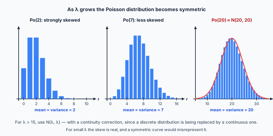
Three Poisson bar charts: Po(2) strongly skewed to the right, Po(7) less skewed, and Po(20) nearly symmetric with the normal curve N(20, 20) fitting it closely.
As \( \lambda \) grows the Poisson loses its skew; for \( \lambda > 15 \), \( \mathrm{N}(\lambda, \lambda) \) is a good approximation.

✏️Worked example

Calls arrive at a small office at a mean rate of 3.5 per hour, and may be modelled by a Poisson distribution. (a) Find the probability that exactly 2 calls arrive in a given hour. (b) Find the probability that at least 3 calls arrive in a given hour. (c) Find the probability that at most 4 calls arrive in a 2-hour period. (d) Separately, 0.4% of the components in a large batch are faulty. A random sample of 500 is taken. Use a suitable approximation to find the probability that at least 3 are faulty, justifying your choice.

(a) \( X \sim \mathrm{Po}(3.5) \):

\[ \mathrm{P}(X = 2) = e^{-3.5}\frac{3.5^{2}}{2!} = 0.030197 \times \frac{12.25}{2} = 0.185 \]

(b) “At least 3” includes 3, so subtract the cases 0, 1, 2:

\[ \mathrm{P}(X \ge 3) = 1 - e^{-3.5}\left(1 + 3.5 + \frac{3.5^{2}}{2}\right) = 1 - 0.3208 = 0.679 \]

(c) The interval doubles, so \( \lambda \) doubles to \( 7 \). With \( Y \sim \mathrm{Po}(7) \):

\[ \mathrm{P}(Y \le 4) = e^{-7}\left(1 + 7 + \frac{49}{2} + \frac{343}{6} + \frac{2401}{24}\right) = 0.173 \]

(d) Here \( X \sim \mathrm{B}(500, 0.004) \). Since \( n = 500 > 50 \) and \( np = 2 < 5 \), the Poisson approximation is appropriate — \(n\) is large and \(p\) is small. So \( X \approx \mathrm{Po}(2) \) and

\[ \mathrm{P}(X \ge 3) = 1 - e^{-2}\left(1 + 2 + 2\right) = 1 - 5e^{-2} = 1 - 0.6767 = 0.323 \]
Check it. The exact binomial value in (d) is 0.3233, so the approximation agrees to four decimal places — that is how well the Poisson does when \(p\) is genuinely small. In (c), the mean over two hours is 7, so “at most 4” asks for a region well below the mean, and 0.173 is duly small. Compare (a) with (b): 0.185 for a single value against 0.679 for a whole tail is the right ordering.
Rescale \( \lambda \), not the answer. In (c), leaving \( \lambda = 3.5 \) gives \( \mathrm{P}(X \le 4) = 0.725 \) — four times too big, and wrong in an obvious direction: 4 calls is a far more demanding ceiling over two hours than over one, so the two-hour answer must be smaller. Doubling the probability instead of the parameter is worse still: it returns 1.451, which is not a probability at all. Rescale \( \lambda \) first and the rest follows.

📝Practise

Work through these, then reveal the answer.

1. \( X \sim \mathrm{Po}(4) \). Find \( \mathrm{P}(X = 3) \) and state the variance.
\( \mathrm{P}(X = 3) = e^{-4}\dfrac{4^{3}}{3!} = 0.018316 \times \dfrac{64}{6} = 0.195 \). For a Poisson the variance equals the mean, so \( \mathrm{Var}(X) = 4 \).
2. Accidents at a junction occur at a mean rate of 1.2 per month. Find the probability that at least one accident occurs in a given month.
\( \mathrm{P}(X \ge 1) = 1 - \mathrm{P}(X = 0) = 1 - e^{-1.2} = 1 - 0.3012 = 0.699 \). "At least one" is almost always fastest as one minus the zero term.
3. Flaws in a roll of fabric occur at a mean rate of 2.5 per metre. Find the probability of exactly 5 flaws in a 3-metre length.
Rescale first: over 3 metres, \( \lambda = 2.5 \times 3 = 7.5 \). Then \( \mathrm{P}(X = 5) = e^{-7.5}\dfrac{7.5^{5}}{5!} = 0.109 \). Using \( \lambda = 2.5 \) here would be the standard error.
4. Two independent machines produce faults at mean rates of 1.5 and 4.5 per day. Find the probability that at most 4 faults occur in total on a given day.
Since the machines are independent, the total is \( \mathrm{Po}(1.5 + 4.5) = \mathrm{Po}(6) \). Then \( \mathrm{P}(X \le 4) = e^{-6}\left(1 + 6 + 18 + 36 + 54\right) = e^{-6}(115) = 0.285 \). The independence is what licenses adding the parameters — say so.
5. For each situation, state whether a Poisson model is likely to be appropriate and why: (i) the number of goals in a football match; (ii) the number of people arriving at a bus stop in the five minutes after a bus leaves.
(i) Reasonably appropriate — goals are rare, occur singly and roughly at random, though the rate is arguably not constant since a team that is behind attacks more. (ii) Not appropriate — arrivals are not independent or at a constant rate, since people time their arrival around the timetable and cluster just before the next bus. The mark is for identifying which condition fails.
6. \( X \sim \mathrm{Po}(30) \). Use a suitable approximation to find \( \mathrm{P}(X < 25) \), justifying your choice.
Since \( \lambda = 30 > 15 \), the normal approximation applies: \( X \approx \mathrm{N}(30, 30) \) with \( \sigma = \sqrt{30} = 5.477 \). "Less than 25" excludes 25, so the boundary moves in to 24.5: \( z = \dfrac{24.5 - 30}{5.477} = -1.004 \), giving \( \Phi(-1.004) = 0.158 \). (The exact Poisson value is 0.157.)

🔗Go deeper — other people’s work

These are external resources, not mine. If one stops working, tell me and everything above it on this page still stands.

  • Seeing Theory (Brown University) — the Poisson process, animated
  • Khan Academy — the Poisson distribution and its derivation from the binomial
  • Desmos — plot \( \mathrm{Po}(\lambda) \) and watch it become symmetric as \( \lambda \) grows