In practice \( \mathrm{f}(x) \) is zero outside some interval, so the integral runs only over that
interval. The normalisation condition is almost always the first line of the solution — it is
how the unknown constant is found.
Probabilities are areas:
\[ \mathrm{P}(a < X < b) = \int_a^b \mathrm{f}(x)\,\mathrm{d}x \]
\( \mathrm{f}(x) \) is not a probability. It is a density, and it may perfectly well
exceed 1 — a density of 4 over an interval of width \( \tfrac14 \) gives an area of 1. Only
the area is a probability. A related consequence:
\( \mathrm{P}(X = a) = 0 \) for every single value \(a\), since an interval of zero width has zero
area. That is why \( \le \) and \( < \) make no difference here, unlike in the discrete case
(S1 4).
These are the discrete formulae with the sum replaced by an integral — the structure is
identical, including “mean of the squares minus the square of the mean”. Compute
\( \mathrm{E}(X) \) first; the variance needs it.
If the density is symmetric about a value, that value is both the mean and the
median, and you can write it down without integrating. Saying so earns the mark and saves a page of
work.
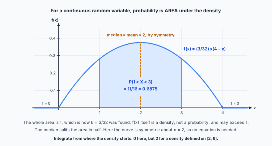
Probability is area under the density: \( \mathrm{P}(1 < X < 3) = \tfrac{11}{16} \), and symmetry puts the median at 2.
Median and percentiles — by area
The median \(m\) is the value that splits the area in half. In 9709 you find it by
direct consideration of an area: integrate the density from the lower end of the
interval up to \(m\) and set the result equal to a half.
Quartiles and percentiles work identically, with 0.25, 0.75 or any other proportion on the right.
The lower quartile satisfies \( \int_a^{q_1} \mathrm{f}(x)\,\mathrm{d}x = 0.25 \), and the
90th percentile puts 0.9 on the right.
Solving usually produces a cubic or a square root. Discard any root lying outside the interval on
which the density is defined — there is exactly one valid answer, so a second root is a signal
to check the range, not the algebra.
The mean and the median coincide only when the density is symmetric. For a
density with a long tail to the right the mean is dragged above the median, exactly as with data in
S1 1. Saying “symmetric, so the median equals
the mean” is a complete answer where it applies, and saves the integration entirely.
Integrate from the start of the interval, not from zero. If the density is
defined on \( [2, 6] \), the median satisfies \( \int_2^m \mathrm{f}(x)\,\mathrm{d}x = 0.5 \).
Starting the integral at 0 quietly includes a region where the density is zero and the limits do
not correspond to the definition — the arithmetic still runs, and the answer is wrong. Write
the interval down before setting up the equation.
A note on \( \mathrm{F}(x) \)
You may meet the cumulative distribution function
\( \mathrm{F}(x) = \mathrm{P}(X \le x) \), the running total of the area from the left. It is a
genuine idea and other courses build the topic on it, but explicit knowledge of it is not
part of the 9709 syllabus — Paper 6 asks for medians and percentiles by area, as
above.
It is still worth knowing what it is, for two reasons. Working out \( \mathrm{F} \) once and
then reading several probabilities off it can be quicker than repeating an integral, and textbooks
written for other syllabuses will assume it. Just do not expect a 9709 question to hand you an
\( \mathrm{F}(x) \) or to ask for one, and do not lose time constructing one when a single
definite integral answers the question in front of you.
✏️Worked example
The continuous random variable \(X\) has density function
\( \mathrm{f}(x) = kx(4 - x) \) for \( 0 \le x \le 4 \), and \( \mathrm{f}(x) = 0 \) otherwise.
(a) Find \(k\).
(b) Find \( \mathrm{E}(X) \) and \( \mathrm{Var}(X) \).
(c) Find \( \mathrm{P}(1 < X < 3) \).
(d) State the median, with a reason.
No distinction is needed between \( < \) and \( \le \) here: a single value has zero
width and so zero area.
(d) The density \( kx(4-x) \) is a downward parabola with roots at 0 and 4, so
it is symmetric about \( x = 2 \). The median is therefore 2, equal to the mean, and
no equation needs solving.
Check it. Re-integrating the density over the whole interval must give exactly
1 — that single line confirms both the value of \(k\) and the integration behind it, and
it is worth doing before anything else depends on them. In (c), 0.6875 is a probability for the
middle half of the range of a distribution peaked at the centre, so a value comfortably above a
half is right. And a variance of 0.8 gives a standard deviation of 0.89 on an interval of width
4 — sensible; anything above about 1.4 would be impossible for a distribution confined to
\( [0, 4] \) and peaked in the middle.
“Median = mean” only when the density is symmetric. In (d) it is
fair because \( kx(4-x) \) is a parabola with roots at 0 and 4, so the sketch is symmetric
about \( x = 2 \) — and the symmetry must be stated to earn the mark, not
silently assumed. Applied to a density that is not symmetric it is simply wrong: question 3
below has mean 2.25 and median 2.38 on the same distribution. When in doubt, sketch the density
and integrate.
📝Practise
Work through these, then reveal the answer.
1. \( \mathrm{f}(x) = kx^{2} \) for \( 0 \le x \le 3 \), zero otherwise. Find \(k\) and \( \mathrm{E}(X) \).
\( \displaystyle\int_0^3 kx^{2}\,\mathrm{d}x = k\left[\frac{x^{3}}{3}\right]_0^3 = 9k = 1 \), so \( k = \frac{1}{9} \). Then \( \mathrm{E}(X) = \frac{1}{9}\displaystyle\int_0^3 x^{3}\,\mathrm{d}x = \frac{1}{9}\cdot\frac{81}{4} = \frac{9}{4} = 2.25 \). The density increases with \(x\), so a mean above the midpoint 1.5 is expected.
2. For the same \(X\), find \( \mathrm{Var}(X) \).
\( \mathrm{E}(X^{2}) = \frac{1}{9}\displaystyle\int_0^3 x^{4}\,\mathrm{d}x = \frac{1}{9}\cdot\frac{243}{5} = \frac{27}{5} = 5.4 \). So \( \mathrm{Var}(X) = 5.4 - 2.25^{2} = 5.4 - 5.0625 = 0.3375 \), giving a standard deviation of 0.581.
3. For the same \(X\), find the median.
Set the area from the lower end of the interval equal to a half: \( \displaystyle\int_0^m \frac{x^{2}}{9}\,\mathrm{d}x = \left[\frac{x^{3}}{27}\right]_0^m = \frac{m^{3}}{27} = 0.5 \). So \( m^{3} = 13.5 \) and \( m = 2.38 \). Here the median exceeds the mean of 2.25 — which is what a density rising towards the upper end should produce, since the long tail is on the left and drags the mean down. Assuming "median = mean" would have been wrong by 0.13.
4. \( \mathrm{f}(x) = \dfrac{3}{x^{4}} \) for \( x \ge 1 \), zero otherwise. Verify that this is a valid density, then find \( \mathrm{E}(X) \) and the median.
The domain is infinite, which is allowed. \( \displaystyle\int_1^{\infty} 3x^{-4}\,\mathrm{d}x = \left[-x^{-3}\right]_1^{\infty} = 0 - (-1) = 1 \) ✓, and \( \mathrm{f}(x) > 0 \) throughout, so it is valid. \( \mathrm{E}(X) = \displaystyle\int_1^{\infty} 3x^{-3}\,\mathrm{d}x = \left[-\tfrac{3}{2}x^{-2}\right]_1^{\infty} = \tfrac{3}{2} = 1.5 \). For the median, \( \displaystyle\int_1^m 3x^{-4}\,\mathrm{d}x = 1 - m^{-3} = 0.5 \), so \( m^{3} = 2 \) and \( m = \sqrt[3]{2} = 1.26 \). The median sits below the mean, as it must for a distribution with a long tail stretching to infinity on the right.
5. For \( \mathrm{f}(x) = \frac{x^{2}}{9} \) on \( [0, 3] \), find \( \mathrm{P}(X > 2) \).
Integrate over the region asked for, remembering the density stops at 3: \( \displaystyle\int_2^3 \frac{x^{2}}{9}\,\mathrm{d}x = \left[\frac{x^{3}}{27}\right]_2^3 = \frac{27 - 8}{27} = \frac{19}{27} = 0.704 \). Most of the probability sits at the upper end because the density is largest there. Taking the upper limit as \( \infty \) rather than 3 is the error to avoid — beyond 3 the density is zero, so there is no area to add.
6. \(X\) is uniformly distributed on \( [2, 10] \), so \( \mathrm{f}(x) = \frac{1}{8} \) there. Find \( \mathrm{E}(X) \), \( \mathrm{Var}(X) \) and \( \mathrm{P}(X < 5) \).
By symmetry \( \mathrm{E}(X) = 6 \) — no integration needed. \( \mathrm{E}(X^{2}) = \frac{1}{8}\displaystyle\int_2^{10} x^{2}\mathrm{d}x = \frac{1}{8}\cdot\frac{1000-8}{3} = \frac{124}{3} = 41.33 \), so \( \mathrm{Var}(X) = 41.33 - 36 = 5.33 \). And \( \mathrm{P}(X < 5) = \frac{5-2}{8} = \frac{3}{8} = 0.375 \), which for a uniform density is just a length ratio.
🔗Go deeper — other people’s work
These are external resources, not mine. If one stops working, tell me and
everything above it on this page still stands.
Khan Academy — probability density functions and continuous distributions
Desmos — plot a density, shade an interval, and read the probability as an area
Seeing Theory (Brown University) — densities and cumulative distributions side by side